

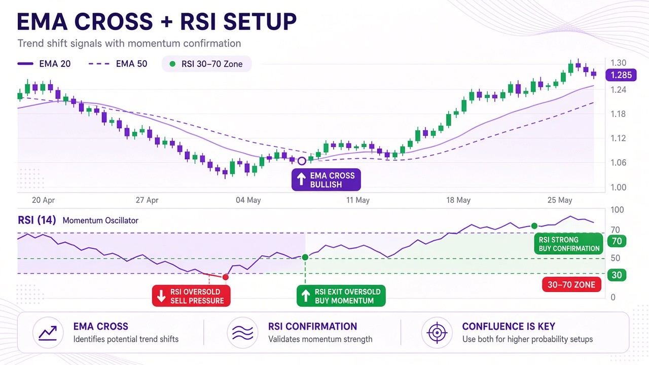
In quantitative trading, technical indicators earn their keep by being explicit and reproducible: the same formula on the same bars yields the same numbers, regardless of mood. EMA tracks trend; RSI gauges momentum strength. Stack them into “dual-core resonance” and the idea is simple — confirm direction first, then use a momentum band to filter crosses that are already overheated or oversold. Below: mechanics, market fit, optional layers, and a Python example aimed at Binance BTC/USDT via CCXT. The code timeframe is 5 minutes; chart titles in the sample sometimes say 1h — trust timeframe = '5m' in the script.
This is not investment advice. Fees, slippage, disconnects, and extreme moves can rewrite live results.
1. What the Dual Core Computes
EMA: a mean that weights recent prices more
EMA (exponential moving average) gives recent closes higher weight, so it reacts to turns faster than a simple moving average (SMA). The recursive form:
EMA_t = α × Price_t + (1 − α) × EMA_{t−1}
where α = 2 / (N + 1), N is the period, and Price_t is the bar’s close. In practice, a short EMA crossing above a long EMA is treated as a bullish turn; crossing below as bearish. The example uses EMA10 and EMA50.
RSI: compressing up/down momentum into 0–100
RSI (relative strength index) compares average gains to average losses over a window. Usual construction:
compute window average gain AvgGain and average loss AvgLoss, then RS = AvgGain / AvgLoss,
RSI = 100 − 100 / (1 + RS)
Textbook reading: RSI > 70 leans overbought (possible pullback); RSI < 30 leans oversold (possible bounce). The dual-core rules do not cling to those extremes; they use milder mid-bands as a “momentum still healthy” filter.
Resonance rules (buy / sell)
- Buy: on the current bar, EMA10 crosses above EMA50 (previous bar was at or below), and RSI sits in 40–70 (trend flipped up, not obviously overbought).
- Sell: on the current bar, EMA10 crosses below EMA50, and RSI sits in 30–60 (trend flipped down, without chopping in deep oversold).
Lone EMA crosses whipsaw easily in ranges; stacking RSI is using momentum to “stamp” the trend signal. That does not erase false signals — it only blocks some clearly hot or cold crosses.
2. What Markets Fit Better
Market type: markets that still trend for a stretch but also chop — crypto names like BTC and ETH often fit that “directional but jumpy” profile. In pure sideways tape, EMA crosses densify; RSI can cut some noise trades but cannot invent a trend that is not there.
Timeframe: source notes also mention 1h / 4h or daily parameter sets (e.g. short-horizon EMA10+EMA50, RSI14; longer-horizon EMA20+EMA100). This example fixes 5-minute candles, ~500 bars — a scalping-style demo. Moving the same dual-core logic to larger periods usually means widening stops and hold time together, not only flipping the timeframe string.
Parameters: in high-vol crypto, some shorten the means further (e.g. EMA5 + EMA20) for faster reaction; whether that helps depends on the symbol and window you care about — there is no universal best set.
3. Three Optional Layers
Stops and targets: fixed percent (e.g. 2% stop) is simple; ATR (average true range) adapts to crypto’s wide swings. Targets can follow a risk/reward ratio (e.g. 1:2) so a correct signal is not given back by weak exits.
Volume filter: require volume above the recent 20-bar mean when a signal fires, which can reduce thin-tape fake breaks. Cost: fewer signals, and long flat stretches in ranges.
Multi-timeframe confirm: e.g. after a 5-minute buy, check that 1h or daily EMA direction agrees; when the higher timeframe disagrees, sit out. Implementation cost: more data and a richer state machine.
4. Python Example: CCXT + EMA/RSI
Rough dependencies: ccxt, pandas, numpy, mplfinance. Flow: batch-fetch BTC/USDT 5m OHLCV → EMA10/EMA50 and RSI14 → dual-core Signal → mplfinance candles with markers → a minimal full-in/full-out sim (no fees or slippage).
import ccxt
import pandas as pd
import numpy as np
import mplfinance as mpf
import time

# Init Binance (public market data)
exchange = ccxt.binance({
    'enableRateLimit': True,
})

# Timeframe string → milliseconds
def timeframe_to_ms(timeframe):
    units = {'m': 60 * 1000, 'h': 3600 * 1000, 'd': 86400 * 1000}
    num = int(''.join(filter(str.isdigit, timeframe)))
    unit = ''.join(filter(str.isalpha, timeframe))
    return num * units[unit]

# Batch-fetch OHLCV
def fetch_ohlcv_batch(exchange, symbol, timeframe, total_needed, max_per_request=200):
    all_ohlcv = []
    timeframe_ms = timeframe_to_ms(timeframe)
    current_time = exchange.milliseconds()
    start_time = current_time - (total_needed * timeframe_ms)
    since = start_time

    while len(all_ohlcv) < total_needed:
        try:
            ohlcv = exchange.fetch_ohlcv(symbol, timeframe, since=since, limit=max_per_request)
            if not ohlcv:
                print("Warning: empty response — empty window or API limit")
                break

            all_ohlcv.extend(ohlcv)
            if len(ohlcv) < max_per_request:
                break

            since = ohlcv[-1][0] + 1
            time.sleep(exchange.rateLimit / 1000)
        except Exception as e:
            print(f"Fetch error: {e}")
            break

    print(f"Bars fetched: {len(all_ohlcv)}")
    return all_ohlcv[:total_needed]

# Pull ~500 bars
symbol = 'BTC/USDT'
timeframe = '5m'
total_needed = 500
ohlcv =  fetch_ohlcv_batch(exchange, symbol, timeframe, total_needed=total_needed)

# Frame
df = pd.DataFrame(ohlcv, columns=['timestamp', 'open', 'high', 'low', 'close', 'volume'])
df['timestamp'] = pd.to_datetime(df['timestamp'], unit='ms')
df.set_index('timestamp', inplace=True)

# EMAs
df['EMA10'] = df['close'].ewm(span=10, adjust=False).mean()
df['EMA50'] = df['close'].ewm(span=50, adjust=False).mean()

# RSI
def calculate_rsi(data, periods=14):
    delta = data.diff()
    gain = (delta.where(delta > 0, 0)).rolling(window=periods).mean()
    loss = (-delta.where(delta < 0, 0)).rolling(window=periods).mean()
    rs = gain / loss
    return 100 - (100 / (1 + rs))

df['RSI'] = calculate_rsi(df['close'])

# Signals
df['Signal'] = 0
for i in range(1, len(df)):
    # Buy: EMA10 crosses above EMA50 and RSI in 40–70
    if (df['EMA10'].iloc[i] > df['EMA50'].iloc[i] and
            df['EMA10'].iloc[i-1] <= df['EMA50'].iloc[i-1] and
            40 <= df['RSI'].iloc[i] <= 70):
        df['Signal'].iloc[i] = 1
    # Sell: EMA10 crosses below EMA50 and RSI in 30–60
    elif (df['EMA10'].iloc[i] < df['EMA50'].iloc[i] and
          df['EMA10'].iloc[i-1] >= df['EMA50'].iloc[i-1] and
          30 <= df['RSI'].iloc[i] <= 60):
        df['Signal'].iloc[i] = -1

df['Buy_Signal'] = np.where(df['Signal'] == 1, df['close'], np.nan)
df['Sell_Signal'] = np.where(df['Signal'] == -1, df['close'], np.nan)

add_plots = [
    mpf.make_addplot(df['EMA10'], color='blue', label='EMA10'),
    mpf.make_addplot(df['EMA50'], color='orange', label='EMA50'),
]

scatter_plots = [
    mpf.make_addplot(df['Buy_Signal'], type='scatter', markersize=100, marker='^', color='green', label='Buy'),
    mpf.make_addplot(df['Sell_Signal'], type='scatter', markersize=100, marker='v', color='red', label='Sell'),
]

all_plots = add_plots + scatter_plots

mpf.plot(
    df,
    type='candle',
    style='charles',
    title=f'{symbol} 1h EMA+RSI Strategy',
    ylabel='Price (USDT)',
    addplot=all_plots,
    volume=True,
    figsize=(15, 10),
)

# Minimal sim
initial_balance = 10000  # USDT
balance = initial_balance
position = 0  # BTC
for i in range(len(df)):
    if df['Signal'].iloc[i] == 1 and balance > 0:
        position = balance / df['close'].iloc[i]
        balance = 0
        print(f"Buy: {df.index[i]}, price: {df['close'].iloc[i]}")
    elif df['Signal'].iloc[i] == -1 and position > 0:
        balance = position * df['close'].iloc[i]
        position = 0
        print(f"Sell: {df.index[i]}, price: {df['close'].iloc[i]}, balance: {balance}")

final_balance = balance + position * df['close'].iloc[-1]
print(f"Initial: {initial_balance}, Final: {final_balance}, Return: {(final_balance - initial_balance) / initial_balance * 100:.2f}%")
Note: the mpf.plot title string says 1h while timeframe = '5m' above — a sample typo; the chart title does not change which bars were fetched. Assigning with df['Signal'].iloc[i] = … can raise SettingWithCopy warnings on newer pandas; production backtesters usually build a signal series then assign once.
5. How to Read the Sample Backtest Number
According to one sample run printout: a buy appeared (e.g. near 2025-03-19 18:20:00, price about 84390.84); starting from 10000 USDT, ending around 10224.75, return about +2.25%. That is a single short window with no fees or slippage — change the window or add real costs and the figure moves; it is not a stable daily wage.
When you read such output, at least ask: how many full round-trips in the sample? What was max drawdown? Were signals clustered in a few hours? After spot-style fees (often a few basis points) and slippage, how much of that 2.25% remains?
6. Code Notes and Improvements
Data: CCXT hits Binance public OHLCV; enableRateLimit and batched since advances reduce rate-limit hits.
Indicators: EMA10 / EMA50 for trend crosses; RSI14 for the momentum band. Buy needs an up-cross with RSI∈[40,70]; sell needs a down-cross with RSI∈[30,60].
Sim book: flat → full buy on signal; long → full sell on signal; open position at the last bar marked to close. No position sizing, no stop module — fine for learning signals, not a live engine.
Possible upgrades: genetic or grid search on parameters; secondary confirms (MACD, Bollinger); separate risk modules for stops, drawdown circuit-breakers, and per-trade risk caps; longer out-of-sample tests before any live use. Black swans and exchange quirks (maintenance, wicks, thin books) still need their own playbook.
7. Takeaway
EMA + RSI dual-core resonance is “trend cross + momentum not too hot/cold.” On directional crypto short horizons it often looks cleaner than naked crosses and is easy to encode for backtests; downsides include lagging in fast one-way moves, or missing a stretch because RSI filtered it out. The sample closes the loop from fetch → chart → crude P&L print — treat it as a research starting point.
Again: for technical learning and strategy discussion only — not investment advice. Size risk yourself, and fold fees, slippage, and capital rules into the model before anything live.